Background Information
| Breed Card | |
| Breed | Leghorn |
| Species taxonomy | Gallus gallus domesticus |
| Classification | Commercial |
| Region | Italy |
| Purpose | Layer |
The Leghorn is a breed that originated in Tuscany of Central Italy. It was initially called as "Italians". Since 1865, the breed has been known as "Leghorn", that is, the traditional Anglicization of "Livorno". Livorno is the port city from which Leghorns were exported to North America for the first time. In Germany, Leghorns are called "Italieners". White Leghorns are commonly used as layer chickens in many countries of the world. It is quite often thought of as an American bird since it was refined and perfected into a stable breed in the United States before being shipped back to Europe.
Leghorns have white earlobes, bright-yellow legs, and large combs and wattles. The breed comes comes in two varieties; the single-combed and the less common rose-combed. A lot of color-varieties are also recognized for the Leghorn. The chicks are easy to rear; feather up quickly and are fast growers. The avarage weights at 7.5 lbs for males and 5-6 lbs for hens. The bantams weigh in at 1kg for males 0.9kg for hens. The Leghorn hen lays anywhere from 280 - 320 eggs (around 55g each) per year without going broody.
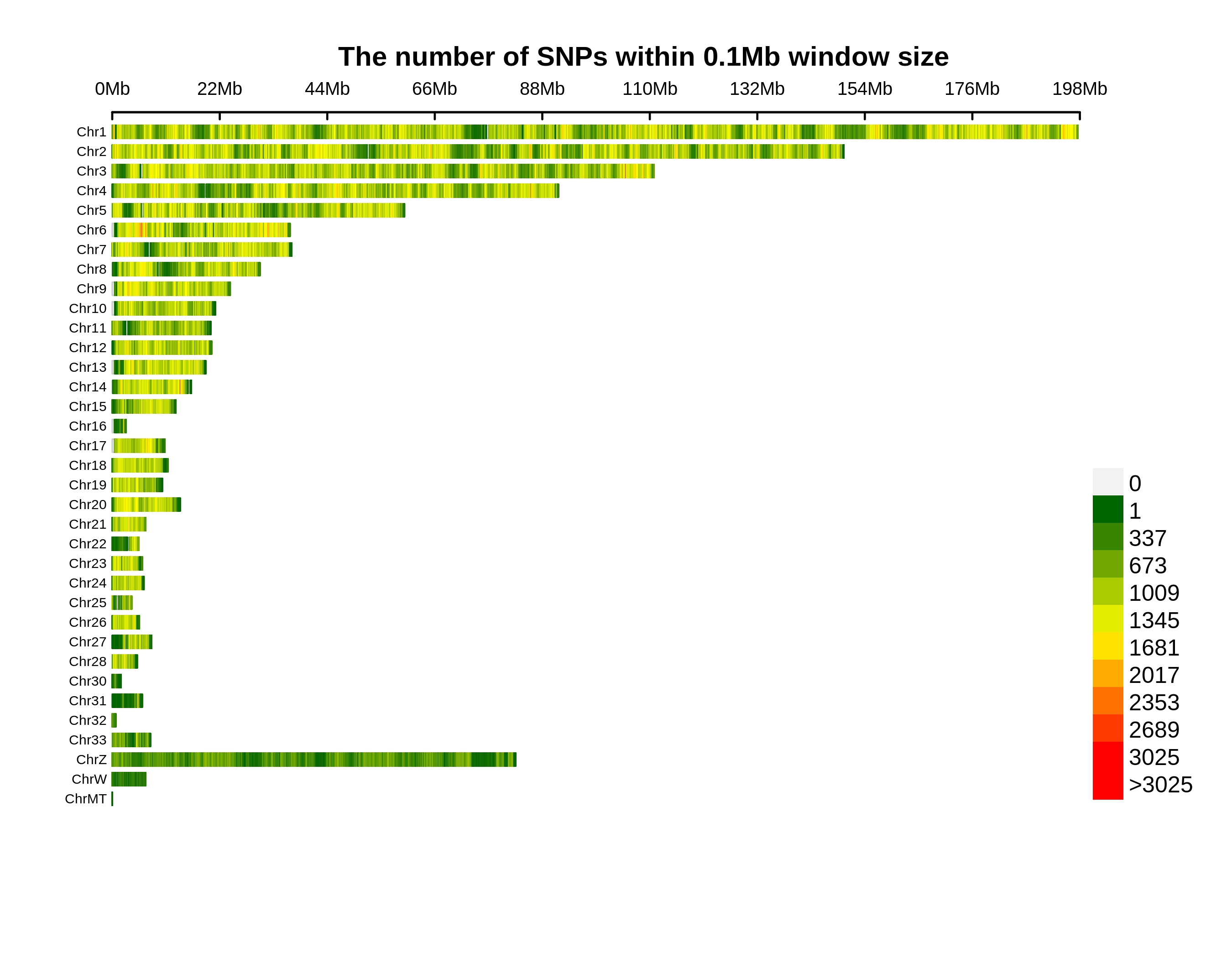
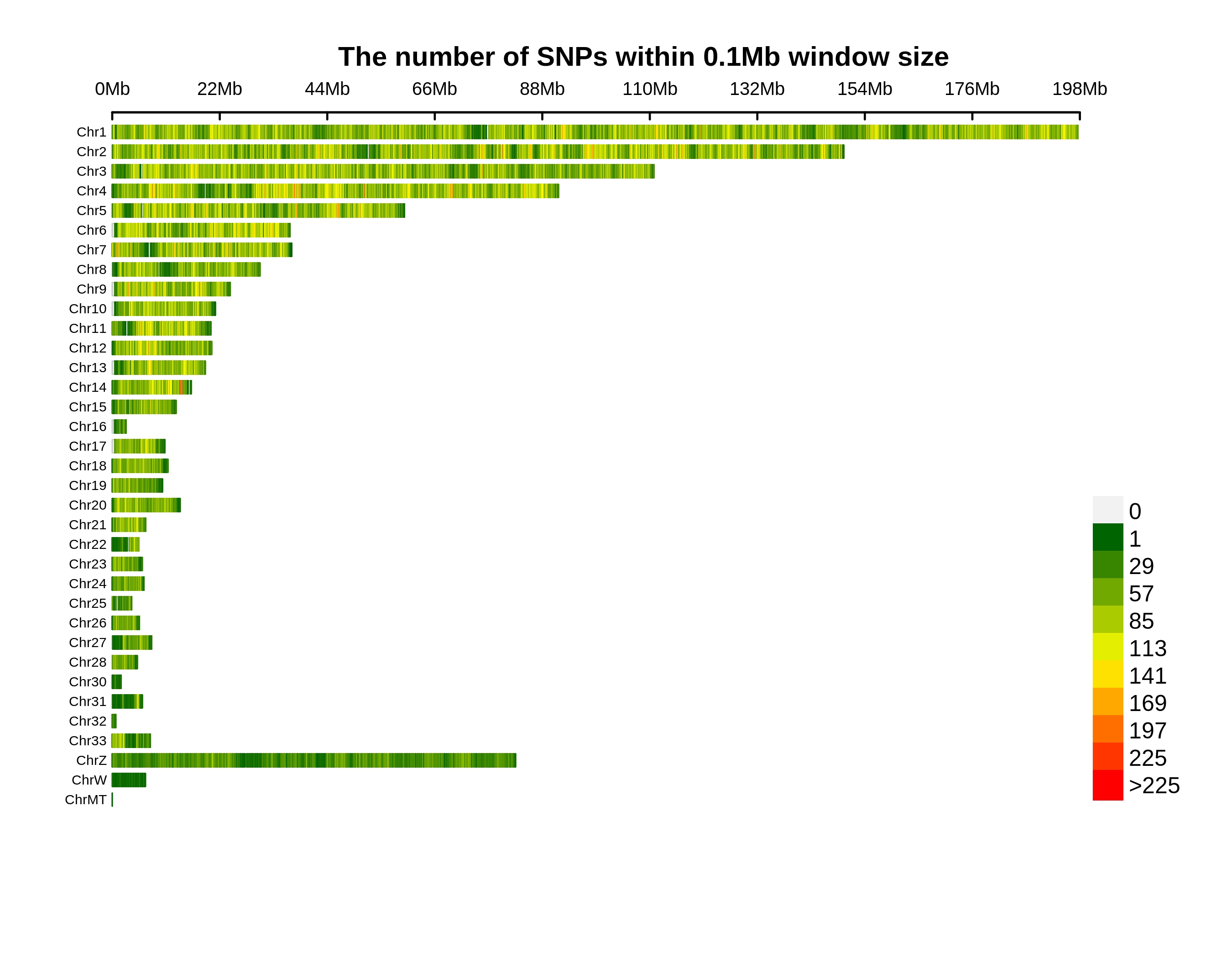
Variants Annotation&Density
| Annotation | Population SNP | Total SNP | Percentage SNP | Population INDEL | Total INDEL | Percentage INDEL |
|---|---|---|---|---|---|---|
| downstream | 130390 | 650455 | 20.046% | 11859 | 104154 | 11.386% |
| exonic;splicing | 26 | 188 | 13.8298% | 0 | 0 | 0% |
| exonic_unknown | 26 | 582 | 4.4674% | 0 | 82 | 0% |
| frameshift_deletion | 0 | 0 | 0% | 630 | 15977 | 3.9432% |
| frameshift_insertion | 0 | 0 | 0% | 510 | 13308 | 3.8323% |
| intergenic | 3006316 | 15129055 | 19.8711% | 253971 | 2238383 | 11.3462% |
| intronic | 3750226 | 17735594 | 21.1452% | 330341 | 2641780 | 12.5045% |
| ncRNA_exonic | 78388 | 400185 | 19.5879% | 6058 | 54342 | 11.1479% |
| ncRNA_exonic;splicing | 62 | 231 | 26.8398% | 7 | 43 | 16.2791% |
| ncRNA_intronic | 758474 | 3728327 | 20.3435% | 67683 | 575920 | 11.7522% |
| ncRNA_splicing | 469 | 2341 | 20.0342% | 59 | 478 | 12.3431% |
| ncRNA_UTR5 | 0 | 0 | 0% | 1 | 18 | 5.5556% |
| nonframeshift_deletion | 0 | 0 | 0% | 362 | 8777 | 4.1244% |
| nonframeshift_insertion | 0 | 0 | 0% | 156 | 4784 | 3.2609% |
| nonsynonymous | 32938 | 336233 | 9.7962% | 0 | 0 | 0% |
| splice_acceptor | 62 | 750 | 8.2667% | 61 | 964 | 6.3278% |
| splice_donor | 96 | 1076 | 8.9219% | 25 | 763 | 3.2765% |
| splice_donor_acceptor | 0 | 0 | 0% | 17 | 45 | 37.7778% |
| splice_UTR5 | 65 | 400 | 16.25% | 7 | 106 | 6.6038% |
| splie_Others | 0 | 0 | 0% | 35 | 654 | 5.3517% |
| startloss | 116 | 671 | 17.2876% | 1 | 51 | 1.9608% |
| stopgain | 341 | 4175 | 8.1677% | 18 | 1252 | 1.4377% |
| stoploss | 66 | 353 | 18.6969% | 6 | 63 | 9.5238% |
| synonymous | 77138 | 548813 | 14.0554% | 0 | 0 | 0% |
| upstream | 131266 | 679592 | 19.3154% | 10321 | 98760 | 10.4506% |
| upstream;downstream | 10768 | 57451 | 18.7429% | 899 | 9367 | 9.5975% |
| UTR3 | 64674 | 361040 | 17.9133% | 6556 | 61415 | 10.6749% |
| UTR5 | 17626 | 112990 | 15.5996% | 1217 | 16935 | 7.1863% |
| UTR5;UTR3 | 424 | 2524 | 16.7987% | 40 | 381 | 10.4987% |
| Total | 8059957 | 39753026 | 20.2751% | 690840 | 5848802 | 11.8116% |
Genetic Differentiation
Summary
Genetic affinities of target population in the context of worldwide populations are measured by pairwise FST between target population and references. Smaller FST value indicates closer relationship. Regions represented by different colors are indicated above.
Genetic Affinity
Summary
Genetic affiliation and population structure are shown by PCA plots. After removing G. g. bankiva, G. g. jabouillei, and some G. g. gallus individuals as outliers to other Red Jungle Fowl, the dataset contains 1,915 samples from domestic chicken and Red Jungle Fowl. User can add any populations with interests to show with the target population under this PCA context by using the item of “Add”.
ADMIXTURE Analysis
Summary
The inference of populations and individual ancestries is revealed by ADMIXTURE clustering. Length of each colored bar represents the proportion of proposed ancestry in the sample. User can add any populations with interests to compare with the target population by using the item of “Add”. The number of proposed ancestries is determined by “which K”.
Runs of Homozygosity
Summary
Runs of homozygosity (ROH) indicates long tracts of homozygous genotypes inherited from identical haplotypes of a common ancestor. Larger populations have fewer, shorter ROH, whereas isolated or bottlenecked populations have more, somewhat longer ROH. Admixture brings the fewest ROH, whereas inbreeding causes long ROH. The level of ROH is measured by number and length. The length of ROH can be defined in “ROH range”. User can add any populations with interests to compare with the target population by using the item of “Add”.
Linkage Disequilibrium Decay
Summary
Linkage disequilibrium (LD) decay is characterized by squared correlations (r²) of all SNPs frequencies against the physical distances between SNPs. User can add any populations with interests to compare with the target population by using the item of “Add”.
Demographic History
Summary
The changes of effective population size through time is inferred by SMC++. User can add any populations with interests to compare with the target population by using the item of “Add”.
Selection
Summary
Selective signals of the target population are detected by different methods. X axis indicates physical position of specific chromosomal region with interests which can be defined by “Region”. The gene annotation is shown below. Y axis of left (YL) indicates the values of Pi-ratio of -log2(πRJF/πTarget) or composite likelihood ratio (CLR) of SweeD. The levels of statistical significance are noted with different colors. Y axis of right (YR) shows the values of Fst (Target vs. Red Jungle Fowl), Pi, or Tajima’s D with blue line with sliding window approach. The genomic window size and step size for Tajima’s D are 5 kb and 5 kb, respectively. The genomic window size and step size for Fst and Pi are 10 kb and 5 kb, respectively. The methods are defined by “Method-YL” and “Method-YR”.
